HiMCM figure choice is a paper-presentation decision, not an official chart-type rule. For a 2026 HiMCM solution — the COMAP contest window runs November 4 to November 17, 2026 — the practical rule is to start from the decision your model is making, then pick the chart that makes that decision legible: an ordered horizontal bar for rankings, a tornado or boundary (Pareto) plot for optimisation, a distribution with the chosen threshold marked for simulation, and a node-link diagram with the decision edges highlighted for network models. COMAP does not publish a mandatory list of chart types, so the matching rules below are a teaching illustration built for teams preparing a written report, not official scoring guidance.
COMAP describes the contest as one in which teams apply mathematics to model and develop a solution to a real-world problem, and it notes that students improve technical writing and communication skills as they prepare a written report, which is then submitted to COMAP for centralized judging. That framing is the entire justification for being strict about figures: a chart that does not advance the reader’s understanding of the recommendation is not neutral — it consumes a slot and competes with the text.
The Reader’s Question: Which Figures Earn a Page?
Teams usually do not have a shortage of plots. They have a shortage of rules for pruning. By the second week, a scripting teammate may have exported twenty or thirty figures, and the writing lead has to decide which three or four go into the body and which single image goes on the summary sheet.
The wrong default is to reason from the output. ‘We ran the simulation, so the simulation histogram goes in.’ The right default is to reason from the decision. If the paper is recommending Option A over Option B, the figure must make the comparison immediate. A pie chart showing percentage shares can be accurate and still fail, because a reader who is trying to see why A beats B has to do arithmetic against a circle. An ordered horizontal bar chart with a marked cutoff does that work for them.
So the selection criterion is one question: does this figure answer the reader’s question about the recommendation faster than the surrounding text could? If the answer is no, the figure is appendix material at best.
Start from the Decision, Not from the Output
Before opening a plotting library, write one sentence on the whiteboard: this model decides X by comparing Y across Z. For a ranking model, the decision is order. For an optimisation model, the decision is a chosen operating point and the trade-off around it. For a simulation model, the decision is a threshold under uncertainty. For a network model, the decision is which edges to include.
That sentence tells you which family of charts will work. If your team is still choosing between model families, the article HiMCM Model Family Choice: Optimization, Simulation, Ranking or Network? is the natural companion, because figure choice is downstream of model-family choice — not the other way around.
Ranking Output: Ordered Bar Chart With an Explicit Cutoff
Multi-criteria problems — the kind that show up in AHP or TOPSIS-style scoring — produce a ranked list of alternatives. The chart that carries the recommendation is a horizontal bar chart sorted by score, with a vertical line marking the acceptance threshold or the natural gap between the top candidate and the rest.
Three rules make the chart work:
- Sort by the score, not alphabetically. The reader must see the order, not reconstruct it.
- Draw the cutoff. A flat bar chart without a threshold line says ‘these are the scores’; a chart with a threshold line says ‘this is the decision’.
- Show uncertainty where it matters. If the top three candidates sit inside each other’s confidence intervals, a plain bar chart is misleading. Use a dot plot with interval whiskers so the reader sees that the ranking is not robust. That honesty is a modelling strength, not a weakness.
COMAP’s previous HiMCM problem Roller Coasters: Develop an Objective Ranking System illustrates this output type; a sorted bar chart with a marked eligibility line is a common effective figure for this family.
Optimisation Output: Boundary or Tornado Plot, Not a Heatmap Dump
Linear, integer, and mixed optimisation problems return a chosen operating point. The temptation is to paste a dense heatmap of the feasible region so the reader ‘sees everything’. In practice this obscures the recommendation, because no single cell in a heatmap tells the reader which constraint was binding or which coefficient the answer depends on.
Two chart types usually do better:
- Tornado plot. A horizontal bar chart of each input parameter’s effect on the objective, sorted by magnitude. It answers ‘which assumption would change my answer?’ in one glance. This is the same reasoning that drives the sensitivity workflow in HiMCM Sensitivity Analysis: Change One Assumption Without Losing the Decision, applied visually.
- Boundary (Pareto) plot. When two objectives conflict — cost against coverage, or speed against emissions — plot the efficient frontier and mark the chosen point. The reader immediately sees the compromise being made. COMAP’s problem Swim, Bike, and Run: Minimize Congestion and Road Closures for a Triathlon is a natural fit for a boundary plot because two objectives genuinely trade off.
Avoid 3D surface plots unless the third dimension carries a comparison the reader is already trying to make; the perspective distortion and occlusion usually cost more clarity than the extra axis buys.
Simulation Output: Distribution With the Chosen Threshold Marked
Monte Carlo output is a distribution, not a number. The figure that earns a slot is a histogram or kernel-density estimate of the chosen metric, with a vertical line for the recommended policy value and a shaded region for the failure or risk tail.
If you are ranking signal-timing plans by average wait time, the summary figure is not a single bar labelled ‘mean = 42 s’. It is the full distribution of wait times under the recommended plan against the baseline, so the reader can see that the mean improvement does or does not come with a fatter tail. Averages hide variance; safety-critical problems are almost always tail problems, and the reader needs the tail.
If the distribution is bimodal, say so in the caption and explain the mechanism — a bimodal outcome usually means two populations are being mixed, which is itself a finding. A short box-plot panel beside the histogram can summarise quartiles, but the histogram stays in the lead because it shows the shape.
Network Output: Node Diagram With the Decision Edge Highlighted
Graph and network problems — routing, assignment, coverage, light-show formations — are best served by a node-link diagram in which nodes are entities and edges are connections. The discipline is to highlight only the edges your algorithm actually selected, and to mute everything else.
Three practical habits reduce clutter:
- Cluster or colour by role, not by aesthetics. Community colouring or role colouring lets the reader see structure without zooming.
- Use a geographic layout when geography is part of the problem. COMAP’s Shop and Ship: Optimal Placement of Warehouses for 1-Day Ground Shipping is a geographic problem; a force-directed layout will look prettier and communicate less than a map with the selected distribution links drawn on top.
- Label the legend by decision. ‘Existing infrastructure’ versus ‘proposed additions’ is more useful than ‘Node A / Node B’.
If the network changes across time — a delivery schedule, a drone formation sequence — a strip of three or four small-map snapshots usually communicates the sequence better than an animation nobody will open.
The Two Figures That Usually Harm the Summary Sheet
Two chart types repeatedly undercut a HiMCM summary sheet, and both fail for the same reason: they ask the reader to do work the text should have done.
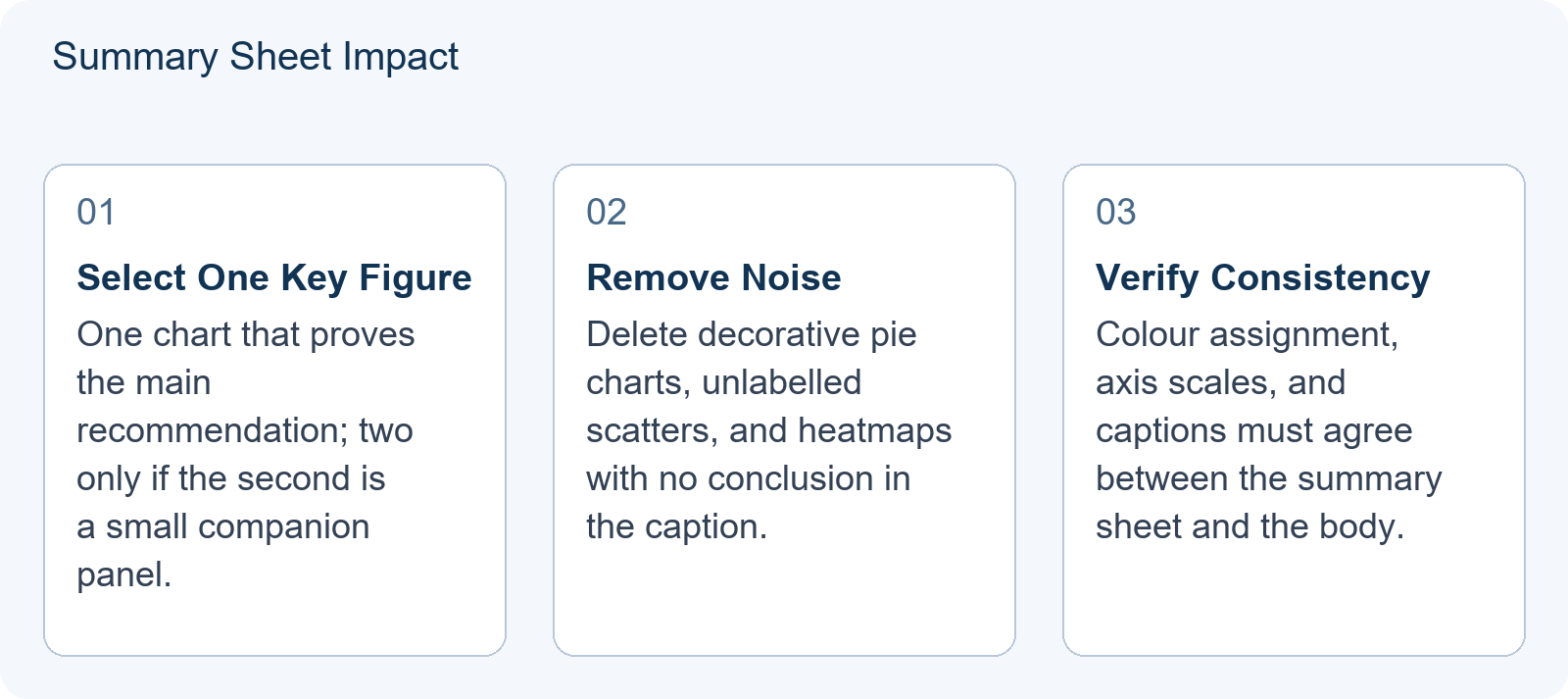
Complex heatmaps without clear axes. Heatmaps are excellent exploratory tools because they compress a lot of comparison into colour. They are poor executive tools because they require the reader to decode a colour scale and a two-way index before reaching any conclusion. If a heatmap must appear, put it in the body with a perceptually uniform scale, labelled axes with units, and a caption that states the conclusion in one sentence.
Pie charts for non-part-to-whole data. Pie charts are often used to show scores, shares of a weighted index, or categorical counts that do not sum to a meaningful whole. That is a category error. Even when the data is genuinely part-to-whole, more than five slices becomes hard to compare. On a summary sheet, an ordered bar chart communicates the same content with less decoding cost.
These are coaching judgments about readability, not official rubric text. COMAP has not published chart-type rules, so treat the paragraph above as a starting position you can defend with your advisor, not a regulation.
Teaching Illustration: Same Result, Two Bad Charts, One Good Chart
This section presents a hypothetical teaching illustration. It is not an official scoring example and does not describe any specific contest paper.
Suppose a model ranks fifty candidate cities for a new facility on cost and accessibility, and the recommendation is the top three. The team has three ways to present this.
Bad chart 1 — the unlabelled scatter. All fifty cities are plotted on cost against accessibility with no labels. The reader sees a cloud and cannot identify the recommended three. The chart is honest and useless.
Bad chart 2 — the pie chart. Each city’s composite score is drawn as a slice of a circle. This implies the fifty scores form a meaningful whole and turns a ranking question into a share question. The reader cannot see order and cannot see the cutoff.
Good chart — the sorted bar chart with a cutoff. Only the top five cities are shown. Two bars per city (cost score and accessibility score, normalised to 0–100) sit side by side, the list is sorted by composite score, and a shaded band marks the acceptable range. The reader sees the recommendation, the margin over fourth place, and the reason the top three win, in under ten seconds.
The lesson generalises. The right figure is not the most complete figure; it is the figure that carries the decision.
A Five-Minute Figure Audit Before You Freeze the Paper
Before the PDF is locked, run this checklist against every figure in the document. Any figure that fails two or more items is a candidate for the appendix or for deletion.
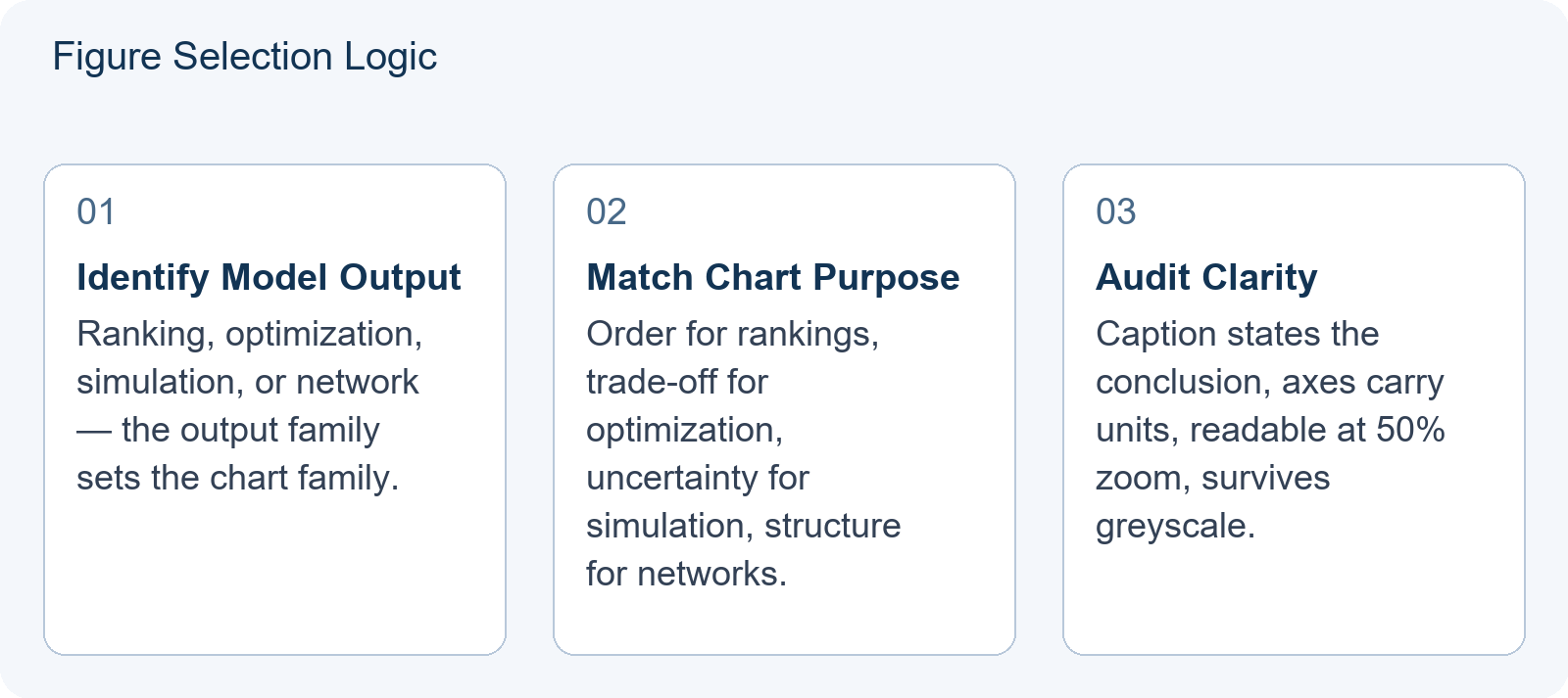
- Does the caption state the conclusion? ‘Mean wait time falls by 12% under Schedule B’ is a conclusion. ‘Wait times’ is a title, not a caption.
- Are the axes labelled with units? ‘Time’ is not a unit. ‘Minutes’ is.
- Is the text readable at 50% zoom? If you cannot read the smallest tick label on a printed page, judges reading on a laptop cannot either.
- Does it survive greyscale? Colour-blind and black-and-white readers are a real part of the audience. If two series are distinguished only by red and green, they will merge.
- Is it referenced in the body text? A figure that is never cited is decoration. Either cite it or remove it.
- Is the colour scheme consistent across the paper? If Figure 1 uses blue for cost, Figure 3 must not reuse blue for time.
Then do the page-envelope check: the summary sheet carries one figure, occasionally two, and no more. Supporting figures live in the body. The reasoning behind the page envelope and the section order is set out in The HiMCM Paper Is the Product: Summary Sheet, Section Architecture and the 25-Page Envelope (2026), and the rhetorical question of what belongs on the summary sheet itself is covered in HiMCM Summary Sheet: Present the Recommendation Before the Technical Detail. Figure choice sits between those two topics: the envelope tells you how many slots you have, the summary-sheet practice tells you what the first slot is for, and this article tells you which chart fills the slot.
Where to Study Figure Conventions in Awarded Papers
The fastest way to internalise these rules is to read awarded papers as visual references rather than as templates. Hanlin’s study materials include methodology notes and reference sets that are independent study aids; they are not official rubrics and should not be treated as such. When you open an awarded paper, look only at its figures for one pass: which chart appears on the summary sheet, which family of chart recurs in the body, and how captions are worded. Then close the paper and apply the format to your own data. This is the same discipline used in How to Study HiMCM Awarded Papers Without Crossing the Plagiarism Line (2026).
If you want a structured way to bring draft figures to a review session, bring one plot per model output along with the one-sentence decision it is meant to support. That converts a conversation about aesthetics into a conversation about whether the figure is doing its job.
General event background is available at Event background.
This is an independent preparation guide, not affiliated with, endorsed by, or sponsored by COMAP.
Frequently Asked Questions
Does COMAP specify exact chart types for HiMCM?
No. The COMAP contest page describes the modelling, problem-solving and writing goals of HiMCM and confirms that solutions are submitted for centralized judging, but it does not publish a mandatory chart-type list. The chart-selection rules in this article are teaching illustrations for communicating results, not official requirements.
How many figures belong on the summary sheet?
As a coaching default, one decisive figure, occasionally two when the second is a small companion panel. The summary sheet is read before the technical detail, so its purpose is to land the recommendation quickly; detailed exploratory plots belong in the body or appendix.
What if my most interesting result is a heatmap?
Keep the heatmap in the body, where a reader inside the argument will invest the time to decode it, and put a simplified derivative on the summary sheet — typically a sorted bar chart or a single contour that isolates the finding. The heatmap stays in the paper; it just does not carry the executive message.