
Real-world problems rarely come with clean, complete datasets. In HiMCM Missing Data scenarios, teams often face gaps due to sensor failures, non-response surveys, or historical record losses. A common mistake is silently dropping rows or filling gaps with arbitrary numbers without explanation. This article outlines a rigorous approach to handling missing values, focusing on transparency and sensitivity analysis rather than pretending the data is perfect.
Understanding Missingness Mechanisms
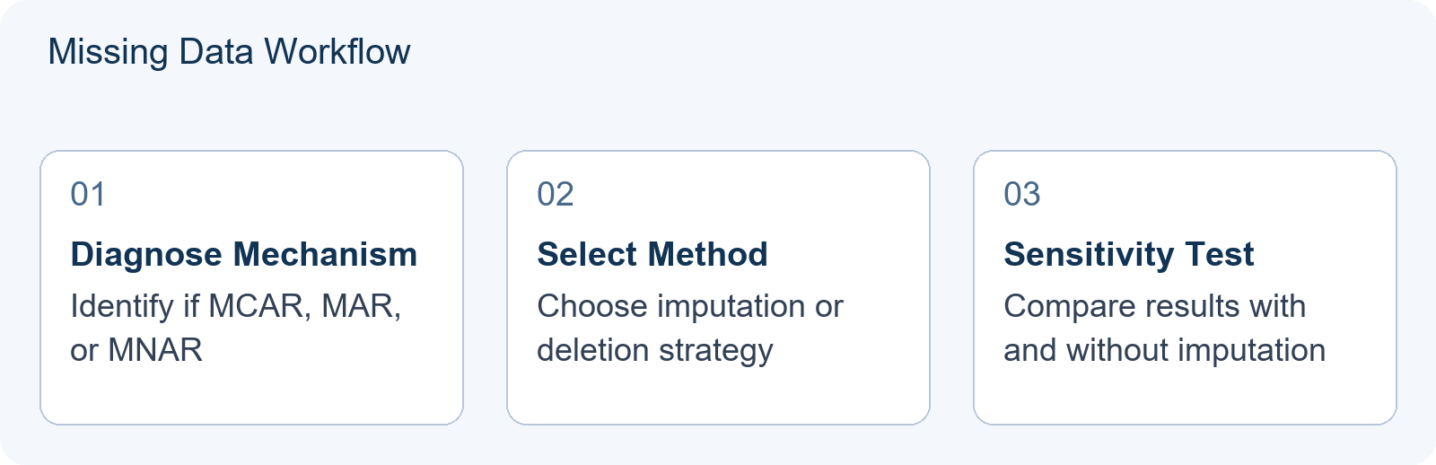
Before choosing an imputation method, you must diagnose why the data is missing. In statistical terms, this falls into three categories:
- Missing Completely at Random (MCAR): The probability of missingness is unrelated to any observed or unobserved variables. Simple deletion might be acceptable here if the sample size remains large enough.
- Missing at Random (MAR): Missingness depends on observed variables. For example, older students might skip a survey question more often than younger ones. Here, imputation using other variables is valid.
- Missing Not at Random (MNAR): Missingness depends on the unobserved value itself. For instance, high-income households might refuse to disclose earnings. This is the most challenging case and requires explicit modeling of the missingness mechanism.
Comparing Imputation Strategies
Once the mechanism is identified, compare different approaches. Do not just pick one; show your team evaluated options. Below is a comparison of common techniques suitable for high school modelling contexts.
| Strategy | Best Use Case | Risk/Challenge |
|---|---|---|
| Listwise Deletion | MCAR data with small missing percentage (<5%) | Loses information; biased if MAR/MNAR |
| Mean/Median Imputation | Numerical data with MCAR/MAR | Reduces variance; distorts distribution shape |
| K-Nearest Neighbors (KNN) | Multivariate data where relationships exist | Computationally heavier; sensitive to scaling |
| Regression Imputation | Strong linear correlation between variables | Overfits noise; underestimates uncertainty |
Documenting Uncertainty
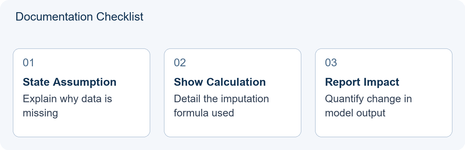
The core principle of good modelling is honesty about limitations. If you impute data, you must document it. Your paper should include a section titled “Data Limitations and Assumptions.” In this section, state exactly which rows were affected, which method was chosen, and why. Crucially, perform a sensitivity analysis. Run your model twice: once with the original incomplete dataset (using only available data) and once with the imputed dataset. Compare the results. If the conclusions change significantly, your model is fragile. If they remain stable, your imputation choice is robust.
This approach demonstrates mathematical maturity. It shows judges that you understand the difference between a point estimate and a confidence interval. You are not hiding the gap; you are quantifying its impact.
Practical Example: Traffic Flow Analysis
Imagine a HiMCM problem involving traffic congestion. You have hourly vehicle counts for 20 intersections, but 3 sensors failed during peak hours. Dropping these hours removes critical peak-load data. Instead, you might use regression imputation based on neighboring intersections. However, you must note that this assumes spatial correlation holds. To test this, you could also try mean imputation from the same intersection’s previous weeks. By presenting both results, you show the range of possible outcomes.
For teams preparing for the contest, practicing this workflow is essential. Review our guide on No Answer Key: How to Test Your Own HiMCM Model With Sensitivity Analysis and Validation to deepen your understanding of validation techniques. Additionally, ensure your team roles are clear before tackling complex data issues, as outlined in How to Build a HiMCM Team in 2026: Four Roles, the Same-School Rule, and What Your Advisor Can Do.
Remember, the goal is not to create a perfect dataset but to build a defensible model from imperfect data. Transparency builds trust in your solution.
Handling MNAR with Pattern-Mixture Models
Missing Not at Random (MNAR) is the most challenging scenario because the probability of missingness depends on the unobserved value itself. Basic implementations of methods like KNN or linear regression often assume Missing at Random (MAR), meaning they may introduce systematic bias if applied blindly to MNAR data. To address this, you can employ pattern-mixture models, which allow you to explicitly model different assumptions about the missing data.
A pattern-mixture model does not try to guess the missing values directly based on observed correlations. Instead, it stratifies the dataset by the pattern of missingness and estimates parameters separately for each group. For example, in a survey about student stress levels where high-stress students are less likely to respond, you create two groups: “Responders” and “Non-Responders.” You then apply different assumptions to the non-responder group’s missing data.
To implement this in HiMCM, follow these steps:
- Define Scenarios: Create three distinct assumptions for the missing values in the non-responder group. A common approach is:
- Conservative: Assume missing values are worse than observed averages (e.g., higher stress scores).
- Neutral: Assume missing values equal the observed average of responders.
- Optimistic: Assume missing values are better than observed averages.
- Run Separate Analyses: Perform your core modelling task (e.g., predicting academic performance) using each of these three imputed datasets independently.
- Report the Range: Do not pick one result. Present the outcomes from all three scenarios. If the conclusion holds across all three, your model is robust to MNAR assumptions. If conclusions flip, explicitly state that the answer depends heavily on the unknown distribution of the missing data.
This method transforms an invisible bias into a visible range of uncertainty. It demonstrates to judges that you understand the structural difference between MAR and MNAR. Unlike simple mean imputation, which shrinks variance and hides the problem, pattern-mixture models expand the confidence interval to reflect true epistemic uncertainty. This is particularly useful in social science or health-related HiMCM problems where self-reporting biases are common. By quantifying the impact of different missingness assumptions, you provide a defensible argument even when the data is fundamentally incomplete.
Frequently Asked Questions
Should I delete rows with missing data?
Listwise deletion is safest when data is Missing Completely at Random (MCAR). If data is Missing at Random (MAR) or Missing Not at Random (MNAR), deletion can introduce bias. In those cases, imputation or modeling the missingness mechanism is often preferred to preserve sample integrity.
How do I know if my imputation is wrong?
You cannot know for sure, but you can test its impact. Perform sensitivity analysis by running your model with different imputation methods. If results vary widely, acknowledge this uncertainty in your paper.
Is it okay to use AI tools for imputation?
COMAP requires disclosure of AI tool usage in the separate AI Use Report. Ensure you understand the algorithm behind any tool so you can defend your modelling choices mathematically.