
When you build a mathematical model for the High School Mathematical Contest in Modeling (HiMCM), you make choices about what matters: which variables to include, which relationships are linear, which parameters have fixed values. A common mistake is treating these choices as facts. Sensitivity analysis tests whether your final recommendation survives when one of those choices changes. It answers the question: if this assumption were different, would I still reach the same decision?
The Core Mechanism: Local Perturbation, Global Consequence
Sensitivity analysis in HiMCM means varying one input or structural assumption while holding everything else constant, then observing whether your output metric—typically an objective function value or a ranked preference—changes enough to alter your recommended action. The goal is not to prove your model is perfect. It is to map the boundary between the region where your decision holds and the region where it fails. A robust recommendation is one that remains optimal across the plausible range of uncertainty in your key assumptions. If a small, realistic change in one assumption flips your decision, you must either gather better data, reformulate the model, or explicitly discuss this fragility as a limitation.
Worked Teaching Illustration: Warehouse Location with Scaled Demand
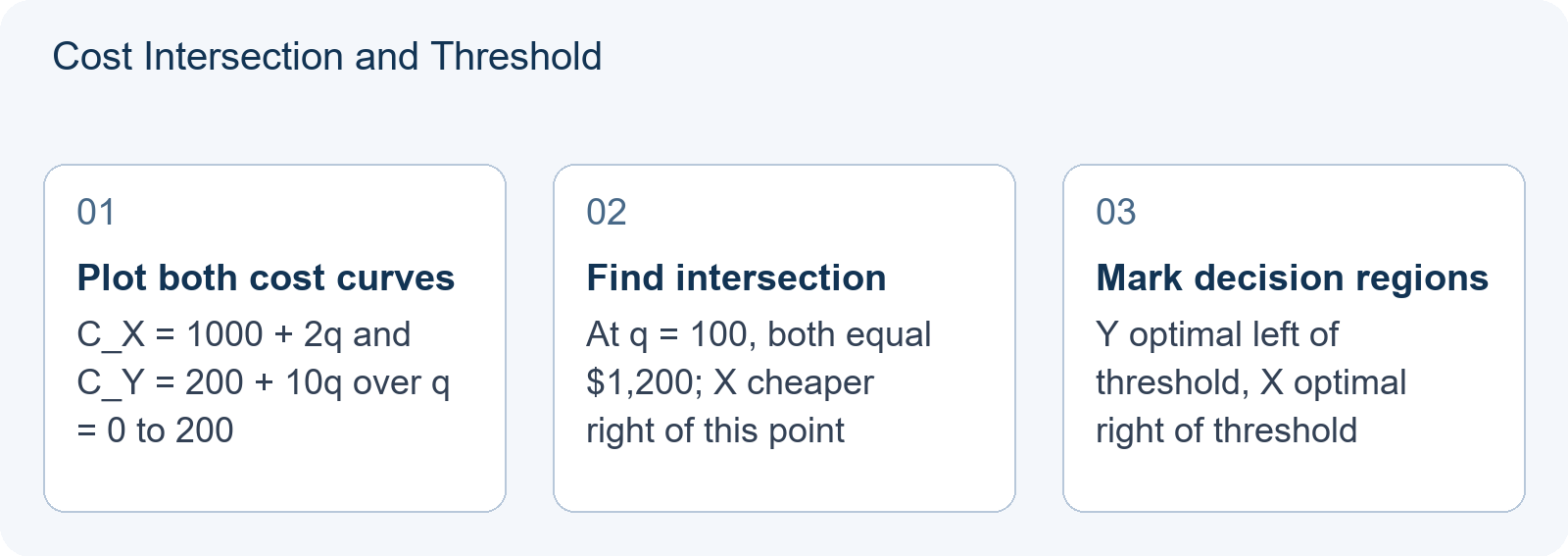
Teaching illustration: hypothetical cost scenario for demonstrating threshold analysis.
Consider a team choosing between two warehouse locations. Location X has a fixed daily cost of $1,000 and a variable cost of $2 per unit shipped. Location Y has a fixed daily cost of $200 and a variable cost of $10 per unit shipped. The team assumes daily demand q = 100 units and selects the cheaper location.
Total daily cost functions:
- C_X(q) = 1000 + 2q
- C_Y(q) = 200 + 10q
At q = 100: C_X = 1000 + 200 = $1,200; C_Y = 200 + 1000 = $1,200. The costs are tied. For any q > 100, C_X < C_Y because the lower variable cost of X overcomes its higher fixed cost. Specifically, at q = 150: C_X = 1000 + 300 = $1,300; C_Y = 200 + 1500 = $1,700. At q = 50: C_X = 1000 + 100 = $1,100; C_Y = 200 + 500 = $700.
The threshold is found by solving C_X(q) = C_Y(q): 1000 + 2q = 200 + 10q → 800 = 8q → q = 100. For all q > 100, X is uniquely optimal; for all q < 100, Y is uniquely optimal. At exactly q = 100, the costs are tied and neither location is uniquely optimal. If demand is confidently expected to exceed 100 units, X is the robust choice. If demand might fall below 100, or if q = 100 is the best available estimate, the team must either gather better forecasts or present both locations as conditionally optimal. The model does not fail; it accurately reveals economic fragility.
Contrasting Case: When Testing Across a Wider Range of Assumptions
A team might test only their assumed value q = 100 and conclude the model is validated. Suppose they also check q = 150 and q = 50, finding X optimal at 150 and Y optimal at 50. They might mistakenly average these or treat them as equally likely without examining the threshold structure. The critical error is stopping at discrete points without deriving the continuous relationship.
Consider a different scenario where the team uses a more complex nonlinear cost for Y: C_Y(q) = 200 + 8q + 0.02q². At q = 100, C_Y = 200 + 800 + 200 = $1,200, tying X again. At q = 150, C_Y = 200 + 1200 + 450 = $1,850, making X clearly preferred. But at q = 200, C_Y = 200 + 1600 + 800 = $2,600 versus C_X = 1000 + 400 = $1,400. The quadratic term accelerates Y’s cost growth. A team that only tests q = 100 and q = 150 might miss that the gap widens favorably for X. Effective sensitivity analysis requires deriving the functional relationship or running dense parameter sweeps, not spot-checking isolated values.
Diagnostic Application: Mapping Robustness Regions
To diagnose your own model, create a structured table that records how your decision responds to each major assumption. For the warehouse case:
| Assumption | Base Value | Range Tested | Decision at Boundary | Robustness Assessment |
|---|---|---|---|---|
| Daily demand q | 100 units | 50 to 150 | X optimal for q ≥ 100 | Medium: depends on demand trajectory |
| Fixed cost X | $1,000 | $800 to $1,200 | Threshold shifts linearly | Ease of calculation does not establish robustness |
| Variable cost Y | $10/unit | $8 to $12 | Threshold shifts with slope | Recalculate the threshold across justified bounds |
If an assumption sits near a threshold where the decision flips, prioritize gathering better data or presenting conditional recommendations. This table demonstrates to judges that you understand your model’s limits.
Interpreting Results for Your HiMCM Paper
Once you identify where your decision holds and where it breaks, your next task is transparent reporting. Dedicate a section to “Sensitivity and Limitations.” Explain why certain parameters are uncertain and how you addressed this. If your decision holds across most plausible scenarios, state this strength explicitly. If it fails under specific conditions, describe those conditions and propose alternative strategies. This demonstrates analytical maturity, a quality valued in HiMCM judging.
COMAP’s official instructions note that teams have a 14-day window to complete their solution, and solutions must be submitted as a single PDF under 20MB. Within that constraint, a clear sensitivity section shows judges that your model is not a black box but a defensible argument.
Practical Preparation and Related Reading
Teams should practice sensitivity analysis before the contest. Review No Answer Key: How to Test Your Own HiMCM Model With Sensitivity Analysis and Validation for workflow guidance. Study HiMCM Missing Data: Comparing Imputation Choices Without Hiding Uncertainty to understand how data gaps interact with parameter uncertainty. Consult HiMCM Baseline Models: Making a Complex Approach Earn Its Place to ensure your sensitivity analysis supports your model complexity rather than undermining it.
From Threshold to Decision: Interpreting the Boundary
The warehouse example reveals a critical distinction in HiMCM modeling: the difference between a mathematical tie and an operational decision. At q = 100, C_X = $1,200 and C_Y = $1,200. The costs are identical. However, the model does not fail here; it accurately identifies the economic break-even point. The fragility is real, not a modeling error. If demand is exactly 100 units per day, both locations are equally optimal. If demand is expected to grow beyond 100 units, Location X becomes strictly superior because its lower variable cost ($2/unit) dominates the higher fixed cost ($1,000/day). Conversely, if demand falls below 100 units, Location Y is cheaper due to its lower fixed cost ($200/day).
Diagnostic Exercise: Evaluating Robustness Under Uncertainty
Teaching illustration: hypothetical scenario for practicing sensitivity interpretation.
Suppose your team’s data source indicates that daily demand q is uncertain but likely falls within the range [80, 120] units. You must decide whether to recommend Location X or Location Y based on this interval.
- Step 1: Calculate costs at the boundaries.
At q = 80: C_X = 1000 + 2(80) = $1,160; C_Y = 200 + 10(80) = $1,000. Location Y is cheaper by $160.
At q = 120: C_X = 1000 + 2(120) = $1,240; C_Y = 200 + 10(120) = $1,400. Location X is cheaper by $160. - Step 2: Assess the decision stability.
The recommendation flips from Y to X as q crosses 100. Since the uncertainty interval [80, 120] straddles the threshold, neither location is robustly optimal across the entire plausible range. - Step 3: Formulate the report conclusion.
Do not arbitrarily pick one. Instead, state: “The optimal choice depends critically on whether projected demand exceeds 100 units/day. For q < 100, Location Y minimizes cost; for q > 100, Location X minimizes cost. Given the uncertainty range [80, 120], we recommend gathering more precise demand forecasts before finalizing the site selection.”
Next Practice Task: Mapping the Sensitivity Surface
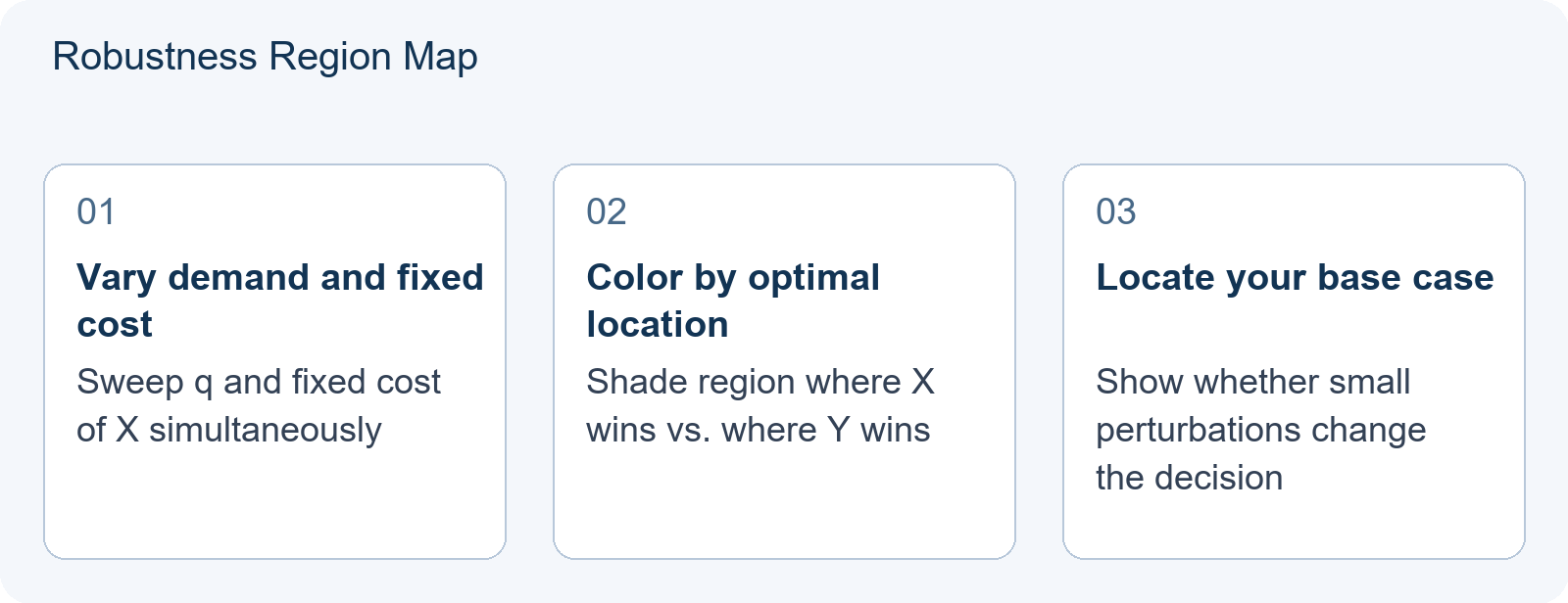
To strengthen your HiMCM paper, move beyond single-point checks. Create a sensitivity table that records how the optimal decision changes as key parameters vary. For the warehouse case, test variations in fixed costs and variable costs separately.
| Parameter | Base Value | Perturbation | New Threshold (q*) | Impact on Decision |
|---|---|---|---|---|
| Fixed Cost X | $1,000 | ±$200 | q* shifts linearly | Higher F_X raises q*, making X less attractive at low demand. |
| Variable Cost Y | $10/unit | ±$2/unit | q* shifts inversely | Lower V_Y raises q*, making Y competitive over a wider range. |
For a checked joint-parameter teaching example, hold demand at q=120. The base costs are X=1000+2×120=1240 and Y=200+10×120=1400, so X is cheaper. Raising only the fixed cost of X to1150 gives X=1390, still below1400. Lowering only the variable cost of Y to9 gives Y=1280, still above1240. Combining both changes gives X=1390 and Y=1280, so Y becomes cheaper. Each isolated change preserves the recommendation; their combination reverses it. These are illustrative perturbations, not measured business ranges.
Structural Sensitivity: When the Model Form Itself Is Wrong
Parameter perturbation tests whether your numbers hold. Structural sensitivity asks a harder question: does your functional form survive? In HiMCM, teams often assume linearity because it is tractable. But if the true relationship is convex—for example, increasing congestion costs—a linear model may produce a decision that looks robust under parameter sweeps yet collapses when the underlying shape changes.
Diagnostic Teaching Illustration: Suppose Location Y’s cost is actually C_Y(q) = 200 + 8q + 0.02q² (convex), not linear. At q=100, C_Y = 1,200, tying X. At q=150, C_Y = 1,850 vs C_X = 1,300; X wins by $550. A team testing only q=100 and q=150 might conclude X is “robustly better.” But at q=50, C_Y = 650 vs C_X = 1,100; Y wins by $450. The cost advantage changes with demand: Y is cheaper by450 at q=50, while X is cheaper by550 at q=150. If your uncertainty interval is [40, 60], X is never optimal. If it is [120, 160], X is always optimal. These are different demand ranges, so their different recommendations do not by themselves demonstrate a structural effect. In fact, the original linear model and this quadratic alternative both tie at q=100 and prefer the same location on either side for nonnegative demand. The model form changes the cost gap here, not the decision boundary.
Actionable Practice: After varying parameters, re-run your decision using an alternative functional form for one key relationship. If the optimal choice flips, your recommendation depends more on model structure than on data precision. Report this explicitly: “In this example, the recommendation survives the alternative cost shape over the same nonnegative demand range, although the estimated savings change. A different alternative would need its own calculation.” This demonstrates awareness that modeling choices are themselves uncertain inputs.
Frequently Asked Questions
How do I know which assumptions to test first?
Start with assumptions that have the largest coefficient in your objective function or those based on the weakest data. In the warehouse case, daily demand q appears in both cost functions with large coefficients, making it the natural first test. As a suggested practice, prioritize assumptions with the largest impact on your objective function or those supported by the weakest data, and document your reasoning.
What if my model’s decision changes at realistic parameter values?
This reveals genuine economic fragility, not a modeling failure. Report the threshold honestly. In the warehouse example, if demand might drop below 100, recommend Y or present both options conditionally. Judges prefer transparency over false certainty.
Does COMAP require specific software for sensitivity analysis?
No. COMAP accepts solutions created with any tools. What matters is the rigor of your analysis and clarity of your explanation, not the software brand. Teams have used Excel, Python, MATLAB, and even hand calculations successfully.